% !TEX program = pdflatex
\documentclass[12pt]{article}
% ---------- Packages ----------
\usepackage[a4paper,margin=1in]{geometry}
\usepackage{amsmath,amssymb,amsfonts,amsthm,mathtools}
\usepackage{microtype}
\usepackage{booktabs}
\usepackage{caption}
\usepackage{subcaption}
\usepackage{enumitem}
\usepackage{siunitx}
\usepackage{csquotes}
\usepackage[hidelinks]{hyperref}
\usepackage{cleveref}
% TikZ / PGFPlots for fully embedded figures
\usepackage{tikz}
\usetikzlibrary{arrows.meta,positioning,calc,patterns}
\usepackage{pgfplots}
\pgfplotsset{compat=1.18}
% ---------- Hyperref colors ----------
\hypersetup{
colorlinks=true,
linkcolor=blue!50!black,
urlcolor=blue!50!black,
citecolor=blue!50!black
}
% ---------- Spacing / Lists / SI ----------
\setlength{\parskip}{0.5em}
\setlength{\parindent}{0pt}
\setlist{nosep}
\sisetup{round-mode=places,round-precision=3}
% ---------- Title ----------
\title{\textbf{Identifying Phase Transitions in Recursive Cognition:\\ From Contradiction to Resonant Growth}}
\author{C.~L.~Vaillant}
\date{October 2025}
% ---------- Document ----------
\begin{document}
\maketitle
\begin{abstract}
This study reformulates the Recursive Generative Emergence (RGE) framework as a measurable dynamical model for recursive cognition. Using the OnToLogic~V1.0 symbolic architecture, contradiction-triggered recursive refinement (CTRR) is defined as a controllable input driving non-linear resonance within recursive feedback systems. The governing equation is
\begin{equation}
\label{eq:core}
\frac{d\hat C}{dt} \;=\; g \;+\; P(t)\,\gamma(t)\,\hat C,
\qquad
P(t) \;=\; \sigma\!\left(k\big(\hat C - C_t\big)\right),
\end{equation}
where $g$ is a baseline adaptation term, $\gamma(t)$ a recursive amplification coefficient, and $P(t)$ a gating function that activates feedback once $\hat C$ exceeds the threshold $C_t$.
\end{abstract}
\section{Introduction}
Recursive feedback processes can exhibit qualitative shifts when internal reference mechanisms exceed a stability threshold. The RGE model describes this transition through the evolution of a coherence function $\hat C(t)$. The objective is to detect this transition empirically as a measurable phase change. We formalize conditions for resonance onset and outline quantitative methods for identifying such transitions across symbolic and statistical substrates.
\section{Model Formulation}
Let $\hat C(t)$ denote internal coherence or structural consistency. System evolution follows
\begin{equation}
\label{eq:model}
\frac{d\hat C}{dt} \;=\; g \;+\; P(t)\,\gamma(t)\,\hat C,
\qquad
P(t) \;=\; \sigma\!\left(k\big(\hat C - C_t\big)\right),
\end{equation}
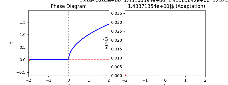
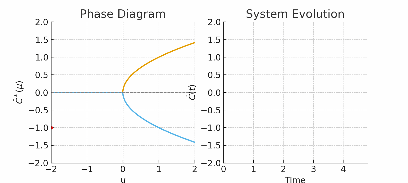
with $g$ baseline adaptation, $\gamma(t)$ the resonance amplifier, and $P(t)$ a smooth gate (e.g., logistic). Crossing $C_t$ induces non-linear feedback leading to accelerated convergence of internal representations.
\subsection*{Key Quantities}
\begin{center}
\begin{tabular}{@{}ll@{}}
\toprule
Symbol & Definition \\
\midrule
$\hat C(t)$ & Coherence / complexity measure \\
$\eta(t)$ & Recursive density (rate of self-queries) \\
$\gamma(t)$ & Resonance amplifier \\
$P(t)$ & Gating function controlling resonance activation \\
$C_t$ & Resonance threshold \\
$\tau$ & Recovery time constant \\
$\Delta\Phi$ & Information / phase gap \\
\bottomrule
\end{tabular}
\end{center}
\section{Experimental Protocol (CTRR)}
The Contradiction-Triggered Recursive Refinement (CTRR) protocol evaluates the relationship between contradiction, recursion, and recovery dynamics:
\begin{enumerate}[label=\arabic*.]
\item \textbf{Initialization:} Stabilize on a defined task set; record baseline.
\item \textbf{Perturbation:} Introduce a controlled contradiction or phase gap $\Delta\Phi$ by altering inputs or symbolic rules.
\item \textbf{Observation:} Record the recovery trajectory of $\hat C(t)$; compute $\tau$ from an exponential (or stretched-exponential) fit.
\item \textbf{Regression:} Assess the scaling relation of $\tau$ versus $1/\Delta\Phi$ across runs and conditions.
\item \textbf{Ablations:} Disable recursion, contradiction handling, or JCB damping to isolate contributions.
\end{enumerate}
\section{Results Framework}
Analyses target phase-transition identification and recovery dynamics.
\begin{itemize}
\item \textbf{Figure~\ref{fig:schematic} (schematic \& observables):} Baseline $\to$ perturbation $\to$ recovery timeline and observable definitions.
\item \textbf{Figure~\ref{fig:recovery} (recovery):} Representative $e(t)$ curves with fitted $\tau$ (with CIs).
\item \textbf{Figure~\ref{fig:scaling} (scaling):} $\tau$ vs.\ $1/\Delta\Phi$ with linear fit and CI band.
\item \textbf{Figure~\ref{fig:jcb} (damping):} Effect of JCB regularization on overshoot, variance, steady-state error.
\end{itemize}
\paragraph{Table 1 (summary statistics).} \Cref{tab:summary} is reserved for aggregated results once experiments are run.
\begin{table}[!t]
\centering
\caption{Summary statistics (placeholders). Report mean and 95\% CI across seeds; $n$ = runs.}
\label{tab:summary}
\begin{tabular}{@{}lcccccc@{}}
\toprule
Condition & $n$ & $\overline{\tau}$ & $R^2\big(\tau \sim 1/\Delta\Phi\big)$ & Slope & Intercept & Notes \\
\midrule
Recursion ON, JCB ON & -- & -- & -- & -- & -- & -- \\
Recursion ON, JCB OFF & -- & -- & -- & -- & -- & -- \\
Recursion OFF & -- & -- & -- & -- & -- & -- \\
\bottomrule
\end{tabular}
\end{table}
\section{Discussion}
Observed transitions from gradual adaptation to accelerated recursive stabilization indicate a distinct dynamical regime governed by the gating function $P(t)$ and threshold $C_t$. Contradictions serve as structured control inputs rather than noise. JCB regularization reduces overshoot and improves recovery characteristics, consistent with a negative-feedback role. The framework is substrate-agnostic and does not assume claims about subjective awareness.
% ============================
\section{Methods}
This section specifies measurement and analysis procedures to support reproducibility.
\subsection{Estimating the Information/Phase Gap $\Delta\Phi$}
We employ multiple estimators to reduce measurement bias:
\begin{enumerate}[label=\alph*)]
\item \textbf{Predictive KL:}
\(
\Delta\Phi_{\text{pred}}
=
\mathrm{KL}\!\big(p_\theta(y\mid x)\,\|\,p^*(y\mid x)\big)
\),
approximated via held-out references or pre-perturbation posteriors.
\item \textbf{Symbolic edit distance:} Minimal graph-edit or proof-edit distance required to restore consistency after perturbation.
\item \textbf{Topological distance:} Bottleneck distance between persistence diagrams computed from evolving concept graphs $G_t$ before/after perturbation.
\end{enumerate}
All estimators are standardized (z-scores) and optionally combined via a weighted average; ablations report each separately.
\subsection{Estimating the Recovery Time Constant $\tau$}
Define an error observable $e(t)$ (e.g., inconsistency rate, deviation from steady state, or $\lvert \hat C(t)-\hat C_\infty\rvert$). Fit
\begin{equation}
\label{eq:expfit}
e(t) \;\approx\; e_0\,\exp\!\left(-\frac{t}{\tau}\right),
\end{equation}
or a stretched-exponential where appropriate, and report confidence intervals.
\subsection{Threshold Detection for $C_t$}
Apply change-point analysis to $d^2\hat C/dt^2$ or to the local slope of $\log e(t)$ to detect transitions consistent with activation of $P(t)$. Report detected threshold locations with CIs and sensitivity to smoothing parameters.
\subsection{Reflexivity Index (RI)}
Define RI as a weighted sum of normalized criteria in $[0,1]$: self-monitoring predictivity, coherence $\hat C$, recursive density $\eta$, contradiction resolution rate, stability $\big(1-\tau/\tau_{\max}\big)$, and ethical regularization efficacy. Weights are preregistered; sensitivity analysis reports robustness to weight variations.
\subsection{Experimental Setup}
We evaluate at least two substrates: (i) LLM + symbolic controller (OnToLogic prompts/rules) and (ii) agent-based simulator with message-passing. Tasks include contradiction resolution, recursive collapse, self-critique loops, and long-horizon repair. Seeds, prompts, and configurations are fixed and versioned.
\subsection{Ablations}
We compare recursion disabled, contradiction handling disabled, and JCB disabled conditions against the full system. Each ablation repeats the perturb--recover protocol and measurement stack.
\subsection{Statistical Analysis}
Primary analysis regresses $\tau$ on $1/\Delta\Phi$ across runs:
\begin{equation}
\label{eq:reg}
\tau \;=\; \beta_0 \;+\; \beta_1 \,\Big(\frac{1}{\Delta\Phi}\Big) \;+\; \epsilon.
\end{equation}
\subsection{Data and Code Availability}
All scripts, prompts, seeds, and raw results will be deposited in an archival repository (DOI) upon completion of experiments.
% ============================
\section{Figures (Embedded TikZ/PGFPlots)}
% ---- Figure 1: Schematic timeline and observables ----
\begin{figure}[!t]
\centering
\begin{subfigure}{0.95\linewidth}
\centering
\begin{tikzpicture}[x=1cm,y=1cm]
% Timeline
\draw[thick,-{Stealth[length=3mm]}] (0,0) -- (12,0) node[below] {time};
% Regions
\fill[blue!10] (0,0.2) rectangle (5,1.2);
\fill[red!10] (5,0.2) rectangle (7,1.2);
\fill[green!10](7,0.2) rectangle (12,1.2);
% Labels
\node at (2.5,0.7) {Baseline};
\node at (6,0.7) {Perturbation};
\node at (9.5,0.7) {Recovery};
% Perturbation marker
\draw[red,very thick] (5,-0.2) -- (5,1.4);
\node[red,below] at (5,-0.2) {$t{=}0$};
\end{tikzpicture}
\caption*{\textbf{Panel A:} Baseline $\rightarrow$ perturbation at $t{=}0$ $\rightarrow$ recovery.}
\end{subfigure}
\medskip
\begin{subfigure}{0.95\linewidth}
\centering
\begin{tikzpicture}
\begin{axis}[
width=\linewidth,
height=5.2cm,
xlabel={time $t$},
ylabel={observable value},
legend style={at={(0.98,0.02)},anchor=south east},
ymin=0, ymax=1.05, xmin=0, xmax=30
]
% C-hat(t)
\addplot[thick,blue] expression[domain=0:30,samples=200]{0.3 + 0.6*(1 - exp(-0.25*(x-2)))*(x>2)};
\addlegendentry{$\hat C(t)$}
% eta(t)
\addplot[thick,orange,dashed] expression[domain=0:30,samples=200]{0.15 + 0.5*(1 - exp(-0.18*(x-2)))*(x>2)};
\addlegendentry{$\eta(t)$}
% contradiction rate
\addplot[thick,red,dashdotted] expression[domain=0:30,samples=200]{0.4*exp(-0.3*(x-2))*(x>2) + 0.05};
\addlegendentry{contradiction rate}
\end{axis}
\end{tikzpicture}
\caption*{\textbf{Panel B:} Observables used for analysis with shaded conceptual bands omitted for clarity.}
\end{subfigure}
\caption{\textbf{Perturbation and response schematic.}}
\label{fig:schematic}
\end{figure}
% ---- Figure 2: Recovery trajectories and tau fits ----
\begin{figure}[!t]
\centering
\begin{tikzpicture}
\begin{axis}[
width=0.9\linewidth,
height=6.2cm,
xlabel={time $t$},
ylabel={$e(t)$},
legend style={at={(0.98,0.95)},anchor=north east},
ymode=log, ymin=1e-3, ymax=1, xmin=0, xmax=40
]
\addplot[thick,blue] expression[domain=0:40,samples=200]{exp(-x/6.0)};
\addlegendentry{run A (fit $\tau{\approx}6$)}
\addplot[thick,red,dashed] expression[domain=0:40,samples=200]{exp(-x/8.0)};
\addlegendentry{run B (fit $\tau{\approx}8$)}
\addplot[thick,green!60!black,dashdotted] expression[domain=0:40,samples=200]{exp(-x/5.0)};
\addlegendentry{run C (fit $\tau{\approx}5$)}
\end{axis}
\end{tikzpicture}
\caption{\textbf{Recovery trajectories and $\tau$ fits.} Representative $e(t)$ curves with exponential fits per \eqref{eq:expfit}.}
\label{fig:recovery}
\end{figure}
% ---- Figure 3: Scaling relation tau vs 1/DeltaPhi ----
\begin{figure}[!t]
\centering
\begin{tikzpicture}
\begin{axis}[
width=0.9\linewidth,
height=6.2cm,
xlabel={$1/\Delta\Phi$},
ylabel={$\tau$},
legend style={at={(0.98,0.02)},anchor=south east},
xmin=0, xmax=10, ymin=0, ymax=12
]
% synthetic scatter
\addplot+[only marks,mark=*,blue] coordinates {(1,2.1) (2,3.0) (3,3.8) (4,5.2) (5,6.1) (6,7.3) (7,8.0) (8,9.1) (9,10.2)};
\addlegendentry{runs}
% linear fit line (example)
\addplot[thick,black] coordinates {(0,1.2) (10,11.2)};
\addlegendentry{linear fit $\;\hat\tau=\beta_0+\beta_1(1/\Delta\Phi)$}
% CI band (illustrative)
\addplot[name path=upper,draw=none] coordinates {(0,1.8) (10,11.8)};
\addplot[name path=lower,draw=none] coordinates {(0,0.6) (10,10.6)};
\addplot[blue!10] fill between[of=upper and lower];
\end{axis}
\end{tikzpicture}
\caption{\textbf{Scaling relation:} $\tau$ vs.\ $1/\Delta\Phi$ with illustrative linear fit and shaded 95\% CI band.}
\label{fig:scaling}
\end{figure}
% ---- Figure 4: JCB regularization effects ----
\begin{figure}[!t]
\centering
\begin{tikzpicture}
\begin{axis}[
ybar,
bar width=14pt,
width=0.9\linewidth,
height=6.2cm,
symbolic x coords={Overshoot, Settling Time, Steady Var},
xtick=data,
ylabel={value (arb.)},
legend style={at={(0.98,0.98)},anchor=north east},
ymin=0
]
\addplot[fill=gray!35] coordinates {(Overshoot,0.35) (Settling Time,0.80) (Steady Var,0.18)};
\addlegendentry{JCB OFF}
\addplot[fill=green!60!black!60] coordinates {(Overshoot,0.18) (Settling Time,0.65) (Steady Var,0.10)};
\addlegendentry{JCB ON}
\end{axis}
\end{tikzpicture}
\caption{\textbf{Effect of JCB regularization.} Reduced overshoot, settling time, and steady-state variance when JCB is enabled (illustrative).}
\label{fig:jcb}
\end{figure}
\section{Conclusion}
Recursive systems exhibit a measurable transition from linear learning to resonant feedback when internal coherence exceeds a critical threshold. This transition can be detected through controlled contradiction experiments and is characterized by an inverse-gap relation between $\tau$ and $\Delta\Phi$. The framework provides a reproducible basis for studying recursion-driven behavior in symbolic and computational systems.
\section*{Supplementary Materials}
Supplement contains: (i) extended derivations for estimator consistency; (ii) additional ablation matrices; (iii) alternative $\tau$ models and diagnostics; (iv) full prompt/rule listings (OnToLogic); (v) detailed parameter tables for all substrates and tasks.
\section*{Acknowledgments}
The author thanks collaborators and reviewers for feedback on methodology and formalization.
\section*{References}
% Manual entries for immediate compilation; switch to BibTeX later if desired.
\begin{enumerate}[leftmargin=2em]
\item Friston, K. (2010). The free-energy principle: a unified brain theory? \textit{Nature Reviews Neuroscience}, 11(2), 127--138. \href{https://doi.org/10.1038/nrn2787}{doi:10.1038/nrn2787}.
\item Tishby, N., Pereira, F. C., \& Bialek, W. (1999). The information bottleneck method. \textit{Proc.\ 37th Annual Allerton Conference on Communication, Control, and Computing}. \href{https://arxiv.org/abs/physics/0004057}{arXiv:physics/0004057}.
\item Tononi, G. (2004). An information integration theory of consciousness. \textit{BMC Neuroscience}, 5(42), 1--22. \href{https://doi.org/10.1186/1471-2202-5-42}{doi:10.1186/1471-2202-5-42}.
\item Vaillant, C. L. (2024). Recursive Generative Emergence: Foundations for Adaptive Symbolic Cognition. Preprint. (Provide DOI/URL upon release).
\end{enumerate}
% BibTeX option (optional)
% \bibliographystyle{unsrtnat}
% \bibliography{rge_phase_transition}
\end{document}